One of the best parts of a project is being able to finally share the results of your analyses. At various points throughout the project, you’ll probably need to share different components of your analyses (code, visualizations, written reports, etc.) with different people. The traditional process may entail performing your analyses in R, exporting your figures and tables, and then manually inserting them into a word document with the written summary of your results. Alongside this written summary, you will then have to share the underlying code and raw data for those who are interested. For collaborators that don’t use R, you will likely have to provide written details on how you processed and analyzed the data, while collaborators who do use R might like to see more about the code you used to run the analyses. Helping to create streamlined summaries for a range of audiences, an essential component of our workflow is the R Markdown (.Rmd) file.
Markdown
After investing time and effort in learning the R coding language, you probably don’t want to hear “time to learn another language”. Before you close this tutorial though, let me assure you that Markdown is not only simple, but extremely powerful when used with R analyses. Markdown is a simple “markup” language used to format documents. R Markdown integrates R code within this formatting framework, allowing you to more efficiently integrate code, visualizations, and written reports. You might imagine that this would be useful for more than just written reports, and indeed, R Markdown can be used to create a wide variety of outputs, including presentation slides and web pages. This tutorial will cover just the basics of integrating a markdown document into your analyses, but you can see here for a more in depth description of R Markdown documents.
Quarto
R Markdown files are fairly specific - it’s assumed that the code you integrate into the files is R code. As projects become increasingly multi-lingual though, the ability to run code from other languages (e.g. Python) in these reports becomes increasingly useful. Recently, a new markdown publishing system called Quarto has provided this capacity. Along with some refined aesthetic capabilities, the ability to run code from languages other than R makes this system worth checking out. Similar to R Markdown, Quarto docs can be used to create a wide range of produces. The website these tutorials are hosted on, for example, was created using Quarto.
Setting up your R Markdown
In RStudio, a new R Markdown file can be created in the same way as a new script, using the page icon in the top left corner of the window. You’ll notice a number of options in the drop-down menu, which can be explored at your leisure. When you create a new Markdown file you’ll be presented with a series of fields and options. Title and Author can be filled in as appropriate. You can input a static date, or choose to use the current date each time you knit (i.e. - run the code for) the document. There are three primary outputs for a markdown file: an HTML, PDF, or Word document. Each come with their own advantages, some of which will be explored in this tutorial. Also, don’t be overly concerned about what you enter into these fields or which options you select - all of these can be changed using the first key component of the markdown file, the YAML.
YAML (Yet Another Markup Language)
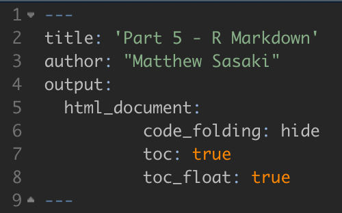
The YAML appears at the top of markdown files and will set key parameters of the document. Some key components of the YAML are explored below. After so much time working with R syntax, the YAML may appear strange, and almost human-readable. This is by design. However, while these sections are typically easier to read, they are just as sensitive to formatting (if not more so) than R code. If you edit the YAML, you should be careful to follow the indentation levels of the various components.
Text Formatting
One of the main reasons to use an R Markdown file is Markdown itself - simple text formatting that looks great. The basic components of a markdown doc are:
Plain text. Entered just as you would with any word processor.
Headings. These are indicated using “#”. Different levels of headings are indicated by different numbers of “#” (Heading level 1 - #, heading level 2 - ##, heading level 3 - ###, etc.).
Bolded and italicized text. To bold text, put two asterisks on either end. To italicize, use just one asterisk.
Other forms of text formatting and customizing the page layout are also possible, with a little more know-how.
Code Chunks
The other reason R Markdown documents are so powerful is the direct integration of R code. These ‘chunks’ of code are what really drive the utility of a markdown document. These chunks of code are run every time you ‘knit’ (run the code for) the document. Take a second to figure out the keyboard shortcut to insert a new code chunk. On a mac, it’s ‘command + option + i’.
The code in a code chunk generally runs just like code in a regular script window. You can name and store objects, create plots, print tables, etc. etc. Objects stored in the environment in one chunk carry through to following chunks.
When you create a new code chunk, by default it assumes you’ll be writing in R (indicated by the {r} at the top of the chunk). You can change this, but we won’t cover that in these tutorials. This header space also allows you to manipulate aspects of the chunk output. There are several key parameters to keep in mind.
echo - T or F. Indicates whether the code in the chunk should be displayed in the knit document above the output of the chunk.
message - T or F. Indicates whether any message outputs from the code in the chunk should be displayed alongside other outputs.
warning - T or F. Indicates whether any warnings generated by the code in the chunk should be displayed alongside other outputs.
fig.width / fig.height - Sets the output dimensions of any figures output by the code chunk (e.g. - ggPlot objects). There are several ways to set these dimensions. The easiest is to provide the dimensions in inches (ex - fig.width = 8). If you know the dimensions of the page you’re working with, this is fairly intuitive.
fig.cap - Allows you to provide a caption for a figure. When set in this way, the caption will display in a nicely formatted way, alongside (auto generated) figure numbers. That markdown will automatically number the figures in consecutive order can be extremely helpful if you’re moving components of a report around, or have to add a new figure to the middle of the document. You can even set it up so that the references to the figure in the main text are updated as well! We’ll discuss how to do this below.
One general note that’s important for both general organization and some of the more useful functions of the R Markdown document, you should give each code chunk a short and informative name. This is specified in the chunk header - {r chunk-name, message = F, warning = F, etc.}
Notice that spaces are not allowed in the chunk name. Instead, you should use a dash (avoid using underscores). Also notice that you do not need a comma after ‘r’, but you do need one after the chunk name before the rest of the options.
The chunk name does a couple useful things. First, it allows you to more easily navigate through the document. At the bottom left of the script window, you’ll find a tool to navigate to different sections of the document. This keeps track of the different headings included in the text as well as the different chunks in the document. Chunk names are also used as figure names if you’re automatically storing figures generated by the document. Finally, these chunk names allow you to refer to figures, tables, etc. in the text. Referring to chunks instead of typing out figure or table numbers can be useful if the structure of the document (order of the figures and tables) is still in flux. Normally, if you were to add in a figure or table to the middle of a document, or re-arrange the existing figures and tables, you’d have to manually correct all the references to figures and tables in the text. This is tedious, and it’s easy to miss something, leading to confusion for readers.
To refer to a figure or table from a code chunk, we can use a ‘\@ref’ statement. For example, if you wanted to refer to a figure generated in a chunk called ‘temp-plot’, you’d include this in the main text: “Figure \@ref(fig:temp-plot)”. Every place that statement is included will be automatically numbered to match the order of the figures in the document. You can do the same for tables by replaced ‘fig:’ with ‘tab:’.
Inline R Code
In addition to the code chunks, you can run R code right in the main text of an R Markdown document. For example:
There are currently 25 documents in the directory used to create this website. Of those, 5 are markdown files.
While this reads like normal text, if you were to look at the markdown file, you’d see this:

By including the R code directly in the text like that, the information on the total number of files and the number of R markdown files is kept up to date. This is a powerful tool when paired with the project folder setup. More than just keeping track of the number of files (although this can be useful too), inline code can present updated statistical results (p-values, correlation coefficients, etc.), or descriptions of the findings (which group has the largest trait value, which sampling site has the lowest latitude, etc.). You can’t completely automate the results section of a manuscript, but when used carefully, inline code can help you keep your reports and manuscripts up to date!
Making your own contributions
As you work on further developing your R skills, you might come across topics that would be useful to expand on or include in these tutorials. Here is a great opportunity for you to contribute to the tutorials. The website is hosted on GitHub, just like the data analytic projects we work on, and you should be able to suggest changes using the same pull request approach we’ve discussed elsewhere on this site.


